[ Generative Models Diffusion] Dataset Generation For Recognition

Introduction

As far as we know, discriminative models always require a large amount of labeled data in general. The deep learning success in previous decay is also based on labor-intensive annotations and crawled images for training. Nowadays, there exist few research works to overcome the need for composing a training dataset manually, but their success is limited. We got started ice-breaking such a limitation. We hypothesize that if we can generate a sample from \(p_{\theta}(x)\) with high fidelity and diversity, then a performance of a trained discriminative model on synthetically generated samples meets that of the counterpart model trained on real data. By referring to the current notable improvement to mimic sampling on true distribution with Diffusion Probabilistic Models (DPMs), we adopted the DPM to generate a training dataset for recognition.

Latent Variable Models (LVMs), and Diffusion Probabilistic Models (DPMs)

Inspired by the diffusion (Brownian motion) as a natural phenomenon in thermodynamics, the diffusion process can be modeled as finding a posterior as the time-introducing LVMs,

\begin{align} \label{diffusionforward} q(x_{T}|x_{t-1}, x_{t-2}, \cdots, x_{1}, x_{0}). \end{align}

The diffusion process is a special case of the Probabilistic Graphical Model (PGM), where the distribution of the latent variable is known, such that

\begin{align} \label{samplelatent} x_T \sim \mathcal{N}(\mathbf{0}, \mathbf{I}). \end{align}

Note that distributions of \(x_0, x_T\) are known in the diffusion context, we can easily compute a sample in the (forward) diffusion process at time \(t\) such that:

\begin{align} \label{computediffusionforward} q(x_{t+1}|x_{T}, x_0) = \sqrt{\bar{\alpha}_t} x_0 + \sqrt{1 - \bar{\alpha}_t}x_T, \end{align}

where \(\alpha_t\) is a constant at \(t\), induced by a beta-scheduler (“linear scheduler” as a common choice). Inherited by the PGM, the reverse diffusion process (the generation process parameterized by \(\theta\)), which finds a likelihood,

\[\begin{equation} q_{\theta}(x_0|x_1, x_2, \cdots, x_{t-2}, x_{t-1}, x_T), \end{equation}\]

can be tractable. To solve this reverse process, Denoising Diffusion Probabilistic Model (DDPM) proposes the \(q_{\theta}\) as a \(\epsilon\)-predictor so that the procedure in training is to be dramatically simple (under the Markov property):

\[\begin{equation} \label{ddpmobjectives} \mathcal{L}_{\text{simple}} := \mathbb{E}_{t, x_0, x_T} \Big [ \| x_T - \epsilon_{\theta}( \underbrace{\sqrt{\bar{\alpha}_t} x_0 + \sqrt{1 - \bar{\alpha}_t}x_T}_{\text{The output of the (forward) diffusion process}}, t ) \|^2 \Big ]. \end{equation}\]

In Eq.[\(\ref{ddpmobjectives}\)], an input to the $\epsilon_{\theta}$ is already acquired in computing the diffusion process (as Eq.[\(\ref{computediffusionforward}\)]).

Sampling \(q_{\theta}(x_0|x_1, \cdots, x_T) \approx p(x_0)\)

First, we sample a latent variable \(x_T\) as Eq.[\(\ref{samplelatent}\)]. To mimic \(p(x_0)\), Authors of DDPM derives followings:

\[\begin{equation} \label{ddpmsample} q_{\theta}(x_{t-1}|x_t, x_0) = \underbrace{ \frac{\sqrt{\bar{\alpha}_{t-1} \beta_t}}{1 - \bar{\alpha}_t} x_0 + \frac{\sqrt{\alpha_t} (1 - \bar{\alpha}_{t-1} ) } { 1 - \bar{\alpha}_t } x_t }_{\mu_t(x_t, x_0)} + \underbrace{ \frac{1 - \bar{\alpha}_{t-1}}{1 - \bar{\alpha}_t} \beta_t \mathcal{N}(0, \mathbf{I}) }_{\Sigma_t}, \end{equation}\]

which means that if we know \(x_0\), computing \(x_{t-1}\) of Eq.[\(\ref{ddpmsample}\)] is tractable via reparameterization trick. The authors of DDMP describe approximating \(x_0\) as in Eq.[\(\ref{ddpmsample}\)] such that:

$$ \begin{equation} \label{approxx0} x_0 := q_{\theta}(x_0 | x_t, x_T) \approx \frac{x_t - \sqrt{1 - \bar{\alpha}_t}\epsilon_{\theta}(x_t)}{\sqrt{\bar{\alpha}_t}}, \end{equation} $$

which regared to as a “input-output reversed” equation of Eq.[\(\ref{computediffusionforward}\)]. The \(x_T\) is the output of our \(\epsilon\)-predictor, \(x_T = \epsilon_{\theta}(x_t)\), where the \(x_t\) is an output for the previous reverse sampling process at \(t+1\).

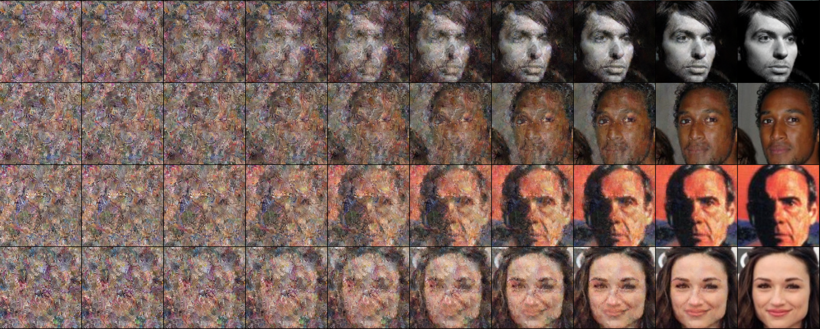
Visualizing intermediate outputs step by step

Forward diffusion process, Eq.[\(\ref{computediffusionforward}\)].

As described above, this forward process can be computed straightforwardly, since we know the distribution of our observation, \(p(x_0)\), and latent, \(p(x_T)\). The right and left-most images are \(x_0\), and \(x_T\), respectively. The remainings are \(x_t\).

Estimating \(x_0\) in Eq.[\(\ref{approxx0}\)].

To estimate the \(x_0\), one needs to sample \(x_{t}\) which is an output of the previous reverse process in the actual sampling (generation) process. However, we can make use of a result of Eq.[\(\ref{computediffusionforward}\)] computed in training for just visualization.

Progressive estimatation of Eq.[\(\ref{ddpmsample}\)].

The following examples are results of Eq.[\(\ref{ddpmsample}\)]. Samples drawn from the normal distribution (left-most images) progressively go to corresponding samples as if they are drawn from the true distribution (right-most images).

Conditional DPM

The conditional DPM is a variant of the diffusion process conditioned on the class label, segmentation mask, CLIP/LAION embeddings, etc. We denote these various conditions as a random variable, \(c\) (for simplicity), where the true distribution of the random variable, \(c\), is known as a part of the observation. Then, previously mentioned Eq.[\(\ref{diffusionforward}\)] changes the form such that

\begin{align} \label{cdiffusionforward} q(x_{T}, x_{t-1}|c, \cdots, x_{1}|c, x_{0}|c). \end{align}

Note the known latent variable, \(x_{T}\), is unchanged under the motivation of diffusion in thermodynamics. Then, final objectives (Eq.[\(\ref{ddpmobjectives}\)]) is changed

\[\begin{equation} \label{cddpmobjectives} \mathcal{L}_{\text{simple}} := \mathbb{E}_{t, x_0|c, x_T} \Big [ \| x_T - \epsilon_{\theta}( \sqrt{\bar{\alpha}_t} x_0 + \sqrt{1 - \bar{\alpha}_t}x_T, c, t ) \|^2 \Big ]. \end{equation}\]

To implement the term, \(\epsilon_{\theta}(x_t, c) := \epsilon_{\theta}(\sqrt{\bar{\alpha}_t} x_0 + \sqrt{1 - \bar{\alpha}_t}x_T, c, t)\), the authors of Stable-Diffusion introduce QKV spatial attention mechanism in their \(\epsilon\)-predictor for conditioning. Another approach is that a diffusion score computed by the \(\epsilon\)-predictor is modified as the amount of gradient of a classifier, \(p_{\phi}(c|x_t)\), additionally introduced (i.e., Classifier-Guidance Diffusion).

\[\begin{equation} \label{classifierguid} \hat{\epsilon}_{\theta}(x_t, c) := \underbrace{\epsilon_{\theta}(x_t)}_{\text{unconditional part}} - \sqrt{1 - \bar{\alpha}_t} \underbrace{\nabla_{x_t} \log p_{\phi}(c | x_t)}_{\text{conditional part}}. \end{equation}\]

The Eq.[\(\ref{classifierguid}\)] could be interpreted as that a diffusion score from unconditional \(\epsilon\)-predictor is changed considering the condition variable \(c\) by a mount of gradient w.r.t. \(x_t\) of \(\log p_{\phi}(c|x_t).\) The authors of the Classifier-Free Guidance (CFG) design their algorithm to get the conditional part in Eq.[\(\ref{classifierguid}\)] without explicit classifier such that:

\[\begin{equation} \label{cfg} \tilde{\epsilon}_{\theta}(x_t, c) := \epsilon_{\theta}(x_t) + w \big (\underbrace{\epsilon_{\theta}(x_t, c) - \epsilon_{\theta}(x_t)}_{\text{the same effect of using explicit classifier}} \big ), \end{equation}\]

where \(w\) is a guidance-scale constant. In this case, we could plug the QKV attention module of the Stable-Diffusion into the term, \(\epsilon_{\theta}(x_t, c)\) to implement. We utilized them to implement our dataset generation for a recognition task.

Latent Diffsion Models (LDMs)

The dimensionality of the random variable, \(x_0\) is the same as the resolution of a generated image, .e.g., \(x_0 \in \mathbb{R}^{3 \times 256 \times 256}\). Such a high dimensional space yields in difficulties to scaling up. To resolve this, the authors of Stable-Diffusion introduce a pretrained encoder-decoder architecture. Specifically, a sample of \(x_0\) is first pass through the pretrained encoder,

\[f_{\text{enc}}: \mathbb{R}^{C \times H \times W} \mapsto \mathbb{R}^{C \times H^{\prime} \times W^{\prime}}, \text{where } H \gg H^{\prime}, W \gg W^{\prime},\]

so that resulting dimensionarity of \(x_0\) is reduced. The forward and reverse diffusion processes are conducted in \(\mathbb{R}^{C \times H^{\prime} \times W^{\prime}}\). To put back to the \(x_t\) to the original image space, the pretrained decoder, \(f_{\text{dec}}: \mathbb{R}^{C \times H^\prime \times W^\prime} \mapsto \mathbb{R}^{C \times H \times W}\), is used. We employed the LDM to implement our dataset generation for a recognition task.

A Dataset Generation via Conditional Diffusion Probabilistic Models (Ongoing)

A common image classification task requires a training dataset that makes our likelihood, \(p(x|c)\), and prior, \(p(c)\), known. We define a discriminative model parameterized by \(\phi\), and then minimize following empricial risk (i.e., the negation of the log-posterior) across samples:

\[\begin{equation} \min_{\phi}\mathcal{L}(\phi; x, c) := -\sum_i \log p_{\phi}(c_i|x_i) \end{equation}\]

The posterior is proportional to the likelihood (parameterized by \(\theta\)) for a given prior,

\[\begin{equation} \label{bayesrule} p_{\phi}(c|x) \propto p_{\theta}(x|c)p(c). \end{equation}\]

This Bayes rule, Eq.(\(\ref{bayesrule}\)), naturally induces our simple hypothesis i.e., if our generator imitates sampling from true likelihood correctly for a given prior \(p(c)\), the performances of discriminators trained on between samples from true likelihood and \(p_{\theta}(x|c)\) are the same. We demonstrate our hypothesis in an application of Face Recognition (FR). The reason behind choosing the FR domain is that the FR is an open-set metric learning task (also regarded as a zero-shot learning task).

Experimental Results

• Experimental Settings: We choose the CASIA-webface dataset (CASIA) composed of about 10 thousand classes (and about 0.5 million face images in total) as our target dataset to train our generator and face recognition network. First, we train our generator via conditional latent diffusion with classifier-free guidance as described above. And then, given the same prior as the CASIA, we sample face images whose number is the same as the CASIA. We denote this as synCASIA. Finally, we train two FR models with the CASIA (Real) and synCASIA (Ours).
• Results for 0.5M (10K x 50) images generated

Methods	Venue	#images (#IDs x imgs/ID)	LFW\(\uparrow\)	CFPFP\(\uparrow\)	CPLFW\(\uparrow\)	AgeDB\(\uparrow\)	CALFW\(\uparrow\)	Avg.\(\uparrow\)	Gap to Real\(\downarrow\)
SynFace	ICCV2021	0.5M (10K x 50)	91.93	75.03	70.43	61.63	74.73	74.75	26.58
DigiFace	WACV2023	0.5M (10K x 50)	95.40	87.40	78.87	76.97	78.62	83.45	13.39
DCFace	CVPR2023	0.5M (10K x 50)	98.55	85.33	82.62	89.70	91.60	89.56	5.65
Ours		0.5M (10K x 50)	99.50	92.97	87.67	92.70	92.40	93.05	0.52
Real		0.49M (10.5K x 47)	99.43	94.54	88.23	92.83	92.60	93.53	0.0

• Results for 1.0M (10K x 100) images generated

Methods	Venue	#images (#IDs x imgs/ID)	LFW\(\uparrow\)	CFPFP\(\uparrow\)	CPLFW\(\uparrow\)	AgeDB\(\uparrow\)	CALFW\(\uparrow\)	Avg.\(\uparrow\)	Gap to Real\(\downarrow\)
DigiFace	WACV2023	1.2M (10K×72 + 100K×5)	96.17	89.81	82.23	81.10	82.55	86.37	9.55
DCFace	CVPR2023	1.0M (20K×50)	98.83	88.40	84.22	90.45	92.38	90.86	4.14
Ours		1.0M (10K×100)	99.43	94.11	88.57	91.50	92.17	93.16	0.40

• Results for 2.0M (CASIA + synCASIA)

Methods	Venue	#images (#IDs x imgs/ID)	LFW\(\uparrow\)	CFPFP\(\uparrow\)	CPLFW\(\uparrow\)	AgeDB\(\uparrow\)	CALFW\(\uparrow\)	Avg.\(\uparrow\)	Gap to Real\(\downarrow\)
Real Only		0.49M (10.5K x 47)	99.43	94.54	88.23	92.83	92.60	93.53	0.0
Real + synCASIA (Ours)		1.0M (20K x 50)	99.63	95.51	90.27	93.53	93.33	94.46	-0.99

Qualitative Results

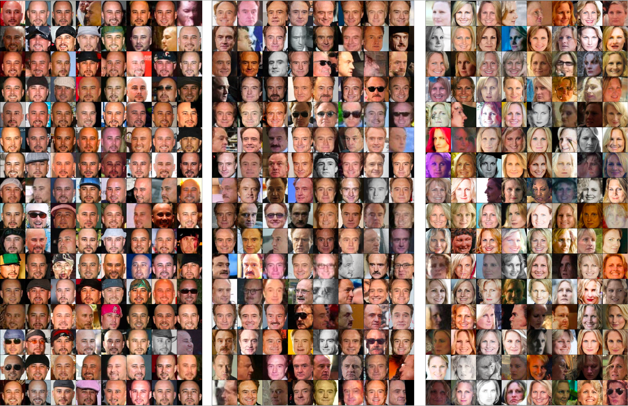
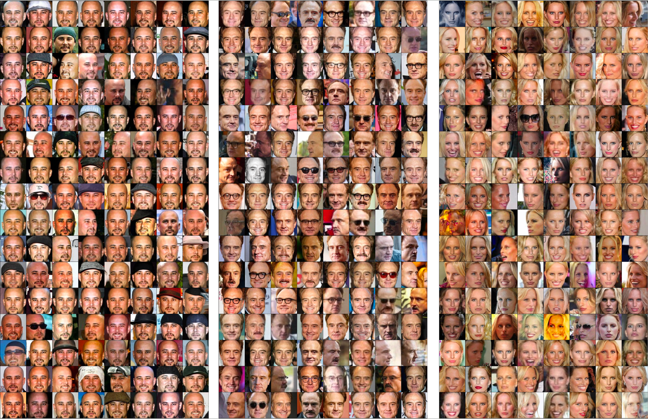
The following results are examples of generated face images. All images are randomly selected (not cherry-picked). There are three groups of images, and all images in a group share the same identity condition.

• Guidance-scale: 1.5

• Guidance-scale: 2.5

Note that we have got started to extend our hypothesis into various vision tasks such as classification, text-vision joint embedding, etc.

Keywords:

Diffusion Probabilistic Models (DPMs), conditional Diffusion Probabilistic Models (cDPMs), Latent Diffusion Models (LDMs), Classifier-Free Guidance (CFG), Dataset Generation